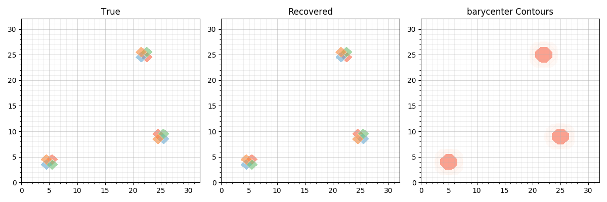
MTW synthetic images

This example generates 3 synthetic sparse images (as regression coefficients) which are fed to random gaussian matrices X. Increasing the Wasserstein hyperparameter increases consistency across regression coefficients.

import numpy as np
import matplotlib.pyplot as plt
from matplotlib import cm

from mtw import MTW, utils
from mtw.examples_utils import (generate_dirac_images, gaussian_design,
                                contour_coefs)


print(__doc__)

print("Generating data...")

seed = 42
width, n_tasks = 32, 4
nnz = 3  # number of non zero elements per image
overlap = 0.
positive = True
n_features = width ** 2
n_samples = n_features // 2

"""Generate Coefs and X, Y data..."""
coefs = generate_dirac_images(width, n_tasks, nnz=nnz, positive=positive,
                              seed=seed, overlap=overlap)
coefs_flat = coefs.reshape(-1, n_tasks)

std = 0.25
X, Y = gaussian_design(n_samples, coefs_flat, corr=0.95, sigma=std,
                       scaled=True, seed=seed)

Out:

Generating data...

set ot params

epsilon = 2.5 / n_features
M = utils.groundmetric2d(n_features, p=2, normed=True)
gamma = utils.compute_gamma(0.8, M)

set hyperparameters and fit MTW

betamax = np.array([x.T.dot(y) for x, y in zip(X, Y)]).max() / n_samples
alpha = 10. / n_samples
beta_fr = 0.35

beta = beta_fr * betamax

callback_options = {'callback': True,
                    'x_real': coefs.reshape(- 1, n_tasks),
                    'verbose': True, 'rate': 1}

print("Fitting MTW model...")
mtw = MTW(M=M, alpha=alpha, beta=beta, sigma0=0., positive=positive,
          epsilon=epsilon, gamma=gamma, stable=False, tol_ot=1e-6, tol=1e-4,
          maxiter_ot=10, maxiter=2000, n_jobs=n_tasks,
          gpu=False, **callback_options)
mtw.fit(X, Y)

Out:

Fitting MTW model...
/home/docs/checkouts/readthedocs.org/user_builds/mtw/envs/latest/lib/python3.7/site-packages/mtw/otfunctions.py:164: UserWarning: Early stop, Maxiter too low !
  warnings.warn("Early stop, Maxiter too low !")
----------------
   it    |   f(t)   |     RMSE(t - t^*) |        AUC - Precision-Recall
       0 | 2.35e+03 |           1.10e-02 |             1.0000
       1 | 2.35e+03 |           1.03e-02 |             1.0000
       2 | 2.35e+03 |           1.02e-02 |             1.0000
       3 | 2.35e+03 |           1.02e-02 |             1.0000
       4 | 2.35e+03 |           1.02e-02 |             1.0000
       5 | 2.35e+03 |           1.02e-02 |             1.0000
       6 | 2.35e+03 |           1.02e-02 |             1.0000
       7 | 2.35e+03 |           1.02e-02 |             1.0000
       8 | 2.35e+03 |           1.02e-02 |             1.0000
       9 | 2.35e+03 |           1.02e-02 |             1.0000
      10 | 2.35e+03 |           1.02e-02 |             1.0000
/home/docs/checkouts/readthedocs.org/user_builds/mtw/envs/latest/lib/python3.7/site-packages/mtw/otfunctions.py:145: RuntimeWarning: invalid value encountered in true_divide
  b = (Q / Ka) ** frac
/home/docs/checkouts/readthedocs.org/user_builds/mtw/envs/latest/lib/python3.7/site-packages/mtw/solver.py:146: UserWarning: Nan found when computing barycenter,
                                         re-fit in log-domain.
  re-fit in log-domain.""")
/home/docs/checkouts/readthedocs.org/user_builds/mtw/envs/latest/lib/python3.7/site-packages/mtw/otfunctions.py:74: UserWarning: Early stop, Maxiter too low !
  warnings.warn("Early stop, Maxiter too low !")
      11 | 2.35e+03 |           1.02e-02 |             1.0000
      12 | 2.35e+03 |           1.02e-02 |             1.0000
Time ot 1.0 | Time cd 2.1

Now we plot the 3 images on top of each other (True), the MTW fitted coefficients and their latent Wasserstein barycenter”””

f, axes = plt.subplots(1, 3, figsize=(12, 4))
coefs = coefs.reshape(width, width, -1)
coefs_mtw = mtw.coefs_.reshape(width, width, -1)
thetabar = mtw.barycenter_.reshape(width, width)[:, :, None]
contours = [coefs, coefs_mtw, thetabar]
titles = ["True", "Recovered", "Barycenter"]
cmaps = [cm.Reds, cm.Blues, cm.Greens, cm.Oranges, cm.Greys, cm.Purples]

for ax, data_, t in zip(axes.ravel(), contours, titles):
    contour_coefs(data_, ax, cmaps=cmaps, title=t)
axes[-1].clear()
contour_coefs(thetabar, ax=axes[-1], cmaps=cmaps,
              title="barycenter Contours")
plt.tight_layout()
plt.show()