Smooth Concomittant MTW

This example performs classification of Handwritten digits using MTW with the concomittant option i.e estimating the standard deviation of each task along with regression coefficients.

import numpy as np
import os
from download import download

from mtw import MTW, utils

from matplotlib import pyplot as plt

print(__doc__)

seed = 42
rnd = np.random.RandomState(seed)

# set n_samples
n_samples = 30
n_features = 240

# take only 3 tasks to run example fast
tasks = [0, 1, 2, 4, 5, 6]
tasks = [0, 1, 2]
n_tasks = len(tasks)
mtgl_only = False
positive = False

Out:

Download data. The images ‘X’ are grouped and sorted. Generate true labels ‘Y’ accordingly

if not os.path.exists('./data'):
    os.mkdir('./data')
url = "http://archive.ics.uci.edu/ml/machine-learning-databases/"
url += "mfeat/mfeat-pix"
path = download(url, ".data/digits.txt", replace=True)
Xraw = np.loadtxt(".data/digits.txt")
Xraw = Xraw.reshape(10, 200, 240)
yraw = np.zeros((10, 2000))
for k in range(10):
    yraw[k, 200 * k: 200 * (k + 1)] = 1.
yraw = yraw.reshape(10, 10, 200)

Out:

Downloading data from http://archive.ics.uci.edu/ml/machine-learning-databases/mfeat/mfeat-pix (1.4 MB)


file_sizes:   0%|                                   | 0.00/1.44M [00:00<?, ?B/s]
file_sizes:   5%|#3                         | 73.7k/1.44M [00:00<00:02, 657kB/s]
file_sizes:  23%|######5                     | 336k/1.44M [00:00<00:01, 829kB/s]
file_sizes:  96%|########################9 | 1.38M/1.44M [00:00<00:00, 1.14MB/s]
file_sizes: 100%|##########################| 1.44M/1.44M [00:00<00:00, 4.17MB/s]
Successfully downloaded file to .data/digits.txt

Each digit corresponds to a task. Reshape data to fit a multi-task learner and split it into a cv and validation set. Here the design matrix X is the same for all tasks.”””

samples = np.arange(200)
samples = rnd.permutation(samples)[:n_samples]
mask_valid = np.ones(200).astype(bool)
mask_valid[samples] = False
ycv = yraw[tasks][:, tasks][:, :, samples].reshape(n_tasks, -1)
yvalid = yraw[tasks][:, tasks][:, :, mask_valid].reshape(n_tasks, -1)
yvalid = np.argmax(yvalid, axis=0)
Xvalid = Xraw[tasks][:, mask_valid].reshape(-1, n_features)
X = Xraw[tasks][:, samples]
X = X.reshape(n_tasks * n_samples, n_features)
scaling = X.std(axis=0)
scaling[scaling == 0] = 1
X = X / scaling
Xcv = np.array(n_tasks * [X])

Compute a Euclidean Ground metric M on a 2D grid.

x = np.arange(16).reshape(-1, 1).astype(float)
y = np.arange(15).reshape(-1, 1).astype(float)

xx, yy = np.meshgrid(x, y)
M1 = abs(xx - yy) ** 2
M = M1[:, np.newaxis, :, np.newaxis] + M1[np.newaxis, :, np.newaxis, :]
M = M.reshape(n_features, n_features) ** 0.5
M_ = M ** 2
M_ /= np.median(M_)

set hyperparams

epsilon = 10. / n_features
betamax = np.array([x.T.dot(y) for x, y in zip(Xcv, ycv)]).max() / n_samples
alpha = 50. / n_samples
beta = 0.075 * betamax
gamma = utils.compute_gamma(0.8, M)

set sigma0, standard deviation lower bound as a percentage of std(Y)

sigma0 = 0.01  # correponds to 1% std(Y)

Create MTW instance and fit

mtw = MTW(M=M_, alpha=alpha, beta=beta, epsilon=epsilon, gamma=gamma,
          sigma0=sigma0, positive=positive, stable=False, tol_ot=1e-5,
          maxiter_ot=15, tol=1e-4, tol_cd=1e-4, maxiter=1000)

mtw.fit(Xcv, ycv)
coefs_ = mtw.coefs_.copy()
ypred = np.argmax(Xvalid.dot(coefs_), axis=1)
errors = (ypred != yvalid).reshape(n_tasks, -1).mean(axis=1)

print(f"Classification error for predicting digits {tasks}:")
print(errors)

Out:

******** WARNING: Stopped early in main loop. *****

You may want to increase mtw.maxiter.
Time ot 13.4 | Time cd 8.0
Classification error for predicting digits [0, 1, 2]:
[0.00588235 0.05294118 0.02352941]

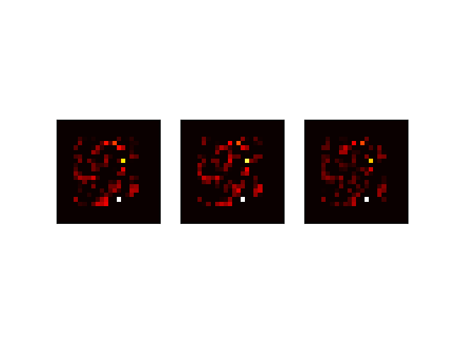
Imshow coefficients

largecoef = np.zeros((n_tasks, 24, 24))
coefs_ = mtw.coefs_.copy()
coefs_ /= coefs_.max(axis=0)[None, :]
coefs_ = np.clip(coefs_, 0, None)
c = coefs_.reshape(16, 15, n_tasks)
c = np.swapaxes(c, 0, 2)
largecoef[:, 4:19][:, :, 4:20] = c

f, axes = plt.subplots(1, n_tasks)
for ax, coef in zip(axes.T, largecoef):
    ax.imshow(np.log(coef.T + 0.1), cmap="hot")
    ax.set_xticks([])
    ax.set_yticks([])
plt.show()